There is currently an intriguing (one might say terrifying) mismatch between the many opinion polls on the coming EU referendum and the betting markets. The poll analysis website http://whatukthinksthinks.org /eu presents a 'poll of polls' that puts Remain and Leave neck and neck at 50%-50%, but on betfair.com the implied probability of a remain vote is (as of 12pm on June 19) 70%.
Tight polls don't necessarily mean the outcome is uncertain. If every poll gave Remain 51% and Leave 49% then we could be quite confident that Remain would win - they only need 50% + 1 vote. When the vote arrives, if 51% say Remain then we can be 100% sure that Remain has won.
But how to compare directly what the polls and betting markets think? The main betting market indicates the probability that Remain or Leave will win, not their respective vote shares. But in a sub-market one can bet on the vote shares themselves, generally in 5% intervals. Using the odds on this market we can find out what the betting market thinks (on average) the Remain vote share will be.
At the moment this sub-market looks like this:

We can take the average of the blue and pink numbers for each percentile as estimates of the reciprocal of the cumulative distribution function (CDF) of the vote share. These are quite coarsely spread at 5% intervals, so to get a better idea what the true CDF looks like we can fit a Beta Distribution to these numbers. A Beta Distribution is a general distribution for describing quantities that can take values between 0 and 1, just like the vote share. In R:
plot(z, dbeta(z, best_parameters$par[1], best_parameters$par[2]), type="n", xlab="x", ylab="p(Vote=x)")

Update 2pm BST June 23. With the polls now open and all opinion polls in there has been a lot of movement on the betting exchanges. Betfair currently give Remain over an 85% chance of victory. With the market looking as below, the expected Remain vote is: 55.5% ± 8.7% (95% CI).

Tight polls don't necessarily mean the outcome is uncertain. If every poll gave Remain 51% and Leave 49% then we could be quite confident that Remain would win - they only need 50% + 1 vote. When the vote arrives, if 51% say Remain then we can be 100% sure that Remain has won.
But how to compare directly what the polls and betting markets think? The main betting market indicates the probability that Remain or Leave will win, not their respective vote shares. But in a sub-market one can bet on the vote shares themselves, generally in 5% intervals. Using the odds on this market we can find out what the betting market thinks (on average) the Remain vote share will be.
At the moment this sub-market looks like this:

We can take the average of the blue and pink numbers for each percentile as estimates of the reciprocal of the cumulative distribution function (CDF) of the vote share. These are quite coarsely spread at 5% intervals, so to get a better idea what the true CDF looks like we can fit a Beta Distribution to these numbers. A Beta Distribution is a general distribution for describing quantities that can take values between 0 and 1, just like the vote share. In R:
x = c(seq(0.4, 0.7, 0.05), 1)#voting percentiles from betfair
iy = c(28.5, 17.5, 5.05, 2.95, 3.83, 11.5, 52.5, 92.5)#betfair odds for each segment
y = 1/iy #Get estimated PDF points from odds
Y = cumsum(y)#get CDF points from PDF
objective_fn <- function(parameters) sum((Y-pbeta(x, parameters[1], parameters[2]))^2) #Create a sqaure error objective to minimise
best_parameters = optim(par=c(1,1), fn = objective_fn) #Get minimising parameters
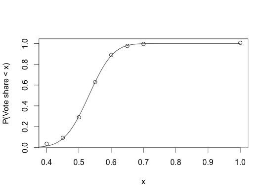
plot(x, Y, xlab="x", ylab="P(Vote share < x)")
z = seq(0,1, length.out=100)
lines(z, pbeta(z, best_parameters$par[1], best_parameters$par[2]))
print(paste(c("Expected Remain vote: ", best_parameters$par[1]/(best_parameters$par[1]+best_parameters$par[2]) )))
Which gives us an output of Expected Remain vote: 0.53, and the figure below:

We can also plot the probability density function to see how likely any given vote share is:
plot(z, dbeta(z, best_parameters$par[1], best_parameters$par[2]), type="n", xlab="x", ylab="p(Vote=x)")
lines(z, dbeta(z, best_parameters$par[1], best_parameters$par[2]))
to give the figure below, which shows that the predicted Remain vote share is peaked around 0.53, and pretty much symmetrically distributed on either side.

So the betting market predicts that the vote share for Remain will be 53%, compared to the polls which put it at 50%. Fitting a Beta Distribution to the data from the market allows us to see what probability the market assigns to any given vote share. We will see in a few days whether the market or the polls are more accurate...
Update 8pm BST June 20. Things have picked up somewhat for the Remain campaign, though uncertainty is still very high. The market currently looks like below, giving a prediction for Remain of: 53.8%± 10.7% (95% CI)

Update 8pm BST June 20. Things have picked up somewhat for the Remain campaign, though uncertainty is still very high. The market currently looks like below, giving a prediction for Remain of: 53.8%± 10.7% (95% CI)

Update 2pm BST June 23. With the polls now open and all opinion polls in there has been a lot of movement on the betting exchanges. Betfair currently give Remain over an 85% chance of victory. With the market looking as below, the expected Remain vote is: 55.5% ± 8.7% (95% CI).
