Sunday, May 27, 2012

Pigeon Navigation (4): Identifying Landmarks

In this last post on pigeon navigation we'll see how we can identify the most important or "information rich" parts of a pigeons flight paths, and then equate these to the landmarks the pigeon uses.

Using the idea that a pigeon learns, and then attempts to follow a memorised `habitual route', we saw in the last post that we could use previously recorded flight paths to predict what future flights by the same pigeon, from the same release site would look like. We could assign a probability to any future path, thus deciding whether it was predictable or not after considering the past flights. The fact that paths typically became more predictable over successive flights was evidence that the pigeons were learning routes home and then sticking to them.

But how does a pigeon learn a route home. It is unlikely that it imagines a perfect line on the ground below it, representing some kind of idealised route it wants to follow. Memorising a complete continuous path, which has an infinite number of locations along it, is hard. Instead, the generally accepted hypothesis is that a pigeon learns its route by memorising a small number of landmarks which act as waypoints. This idea, known as `pilotage', supposes that the bird reaches one landmark, then reorients itself to head for the next until it reaches home.

Can we detect where these landmarks are, using the methodology we've developed so far? Of course we can!

Recall that we previously assumed that a flight path always consisted of 100 recorded positions, starting at the release point and ending at the home loft. We predicted future flights by using these 100 points on each flight path to estimate a habitual route  that the bird was trying to follow. We predict that future flights will also look like this habitual route, plus some variation that changes from flight to flight.

In principle we can choose to ignore some of this data. We can, if we want, choose to estimate the habitual path using only a subset of the data we have. For example, we might choose 10 random points of the 100 we have of each flight, then try to estimate the habitual route from these.

The first important point to understand for identifying landmarks is that such an approach will have varying degrees of success, depending on which points are selected. Consider the figure below


In each case the faint black line is the same simple bell curve. The black dots indicate 3 points on this curve that we are "allowed" to know in order to make a guess what the whole curve looks like. If we draw a smooth line through these three points we get the two red lines. Hopefully it should be clear that the red line on the left is a much better estimate of the bell curve than the very low red line on the right. Therefore, if I wanted to remember 3 points to try and remember the whole of the faint black line, I would better off choosing those on the left, rather than those on the left

But this is exactly what the pigeon has to do! It needs to remember a few landmarks so it can remember the whole of its route home. This suggests the second important point for identifying landmarks: the points that allow best estimation of the habitual route are the same points as the pigeon's landmarks. That means that we assume the pigeon does a good job of choosing the most efficient way to compress its habitual route into a few key points.

Since we can never measure exactly how well we have estimated the habitual route, we do the next best thing and test how well any set of possible landmarks allows us to predict future flights. If we call the subset of times that correspond to landmark locations at t_lm, and the full set of times as t_full, then our task is to choose t_lm to maximise p(x_n+1(t_full) | x_1(t_lm), x_2(t_lm), ..., x_n(t_lm))

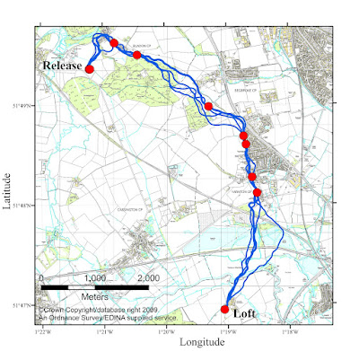
And when we do this, we find landmarks that correspond to recognisable features of both the paths and the landscape beneath, such as below (remember I promised to explain what those red dots were...?)


The landmarks (the red dots) tend to be where the paths are very similar, since here the paths are a very good predictor of the habitual route, where the pigeon flies somewhere unexpected - the apex of the `C' shape - and where the path curves sharply. They also tend to be on the edge of forests and villages, above major roads and obvious features such as a church spire. 

[NB: Those with a machine learning background may see that this process is largely analogous to two other ideas. Active sampling, where we take data in an intelligent way to maximise our predictive power while minimising collection costs, and reduced rank Gaussian process approximations, where we use a subset of data points as `inducing points' to create a lower rank covariance matrix and speed up calculations.]

Monday, May 14, 2012

Pigeon Navigation (3): Habitual Routes

[NB: This post, and the rest of the pigeon posts will be quite mathsy. I've done my best to keep the maths as simple as possible - it should be possible to follow the argument without understanding all the working! On the other hand, if you do want to see the maths done properly, please read it properly formatted!]


Way back when this century was young, the navigation group in Oxford published a series of papers demonstrating that pigeons, when repeatedly released from the same site, would learn to follow the same route back the home loft each time.

If a pigeon is learning and following a route this ought to make its flight patterns predictable. If those flights are getting more and more predictable we should be able to observe that by using a model to predict the flights with increasing accuracy. In other words, we should have a model which gives the probability of a flight path, and that probability should get higher as our predictions get better.

In the last post we saw how to assign probabilities to individual flight paths using a Gaussian process (GP). The precise probability of a given flight path depended on the mean, m, and covariance, S, of that GP. I told you that the covariance dictated how likely the flight path was to be either smooth or wiggly, and we used the straight line between release point and home loft to create the mean. For convenience I'll write down the resulting probability as:

p(x| m, S) = GP(x; m, S)

Now, the reason we chose the straight line path to be the mean was that if we only look at a single path, and we have never seen this particular bird fly before, there is no reason to assume it will fly either one side or the other from this most efficient route. We don't expect the flight path to be perfectly straight, but we don't know beforehand in which direction it will go.

Imagine instead that we had already seen the flight paths below.


Now we should have a very good idea where the next path is going to be, somewhere close to the paths we have already seen. It looks like the pigeon is following a particular route home every time, so its unlikely to suddenly fly directly south from the release point next time. Obviously it doesn't fly exactly the same path every time, but each new flight path is like an imperfect attempt to fly some memorised route.

Lets imagine that we could look into the mind of the pigeon and retrieve exactly what its memorised route looks like. We can call this route h (for 'habitual'). Then we might replace the earlier straight line mean path with the one we now know the bird is trying to fly

p(x | h, S) = GP(x; h, S)


(I'm going to assume for simplicity that we know what  S is, but in practice we would infer it from the data)

Whats more, if we want to find the probability of several flight paths by the same bird, each an attempt to replicate h, we can simply multiply the probability of each path together, because each one is independent if we know h.

p(x1, x2, ...,xn | h, S) = GP(x1; h, S) x GP(x2; h, S) x ... x GP(xn; h, S)


Hang on! Surely those flight paths aren't really independent?! After all, they all look the same. Yes! But the reason they look the same is that they are all attempts to replicate h. They way each path varies around h is independent. All the shared structure in the paths is located in h.

Ok, thats nice, but the problem is that we don't know what h is. All we can see are a few paths that look a bit like h. But never fear - Bayes is here...we can use those flight paths we have actually seen to infer what h is. Recall Bayes' rule which allows use to reverse the order of the conditional probability:

p(h | x1, x2, ...,xn, S)p(x1, x2, ...,xn| h, S) x p(h | S) / p(x1, x2, ...,xn| S)


But we seem to be creating more trouble for ourselves. Now we need to know two more things, p(h | S) and p(x1, x2, ...,xn | S). Are we digging a hole for ourselves?

No! The first of these terms is a prior distribution. It's how likely we think any particular habitual route would be before we see any real paths. So we need to place a probability distribution over a path that could lie anywhere between the release point and the home loft. Thats exactly what we learned how to do in the last post! Before we see any real paths theres no reason to expect the habitual path to be on either side of the straight line, so the probability of h is exactly like a single path on its own, with the straight line as a mean.

p(h | S) = GP(h; m, S)

The second term is the joint probability of the real paths, if we don't know what h is. This can be calculated by integrating over all possible values of h.


∫ p(x1, x2, ...,xn | h, S) x p(h | S) dh


and this is where the theory of Gaussian processes really helps us. Integrals like this are really easy to do (using a few matrix rules...easy is a relative term!) when everything is Gaussian...


∫ p(x1, x2, ...,xn | h, S) p(h | S) dh = ∫ GP(x1; h, S) GP(x2; h, S) GP(xn; h, S) GP(h; m, S) dh


= GP ([x1, x2, ...,xn], [m,m,...,m], Σ)


where those square brackets indicate that we're concatenating the n paths and n copies of the vector m. We have a big new covariance matrix, Σ, which is generated from S. If we want to mathematical details of how we do that I would suggest reading them in this paper (Open access), where it's all properly formatted without the restrictions of html. Here we'll just assume we know the matrix rules for multiplying Gaussian distributions together - check out Appendix A of my thesis if you're interested.

The upshot of all this is that we can calculate a probability distribution, p(h | x1, x2, ...,xn, S), which tells us how likely any given habitual route h is, based on the flight paths we've already seen. Does it work? Well, look at the picture below, showing a set of flight paths from two birds, and the distribution (mean + variance) of the inferred habitual routes. The faint black lines are the flight paths, recorded from GPS. The thick black lines are the 'best guess' of the habitual routes, and the dashed red lines indicate how uncertain these are. The dashed black lines indicate where most future flight paths are expected to lie.


If we can infer what the habitual route is, we should then be able to do exactly what I suggested at the top of this post, and make some predictions about where future flight paths will be, and see if these become more accurate as the birds learn their routes. In fact, we have already done everything we need. We calculated the joint probability of n paths, assuming that we didn't know the habitual route.

 p(x1, x2, ...,xn| S) = GP ([x1, x2, ...,xn], [m,m,...,m], Sigma)

if we want to calculate how probable path xn is, based on the previous n-1 paths, we simply calculate the joint probability of x1, x2, ...,xnand of x1, x2, ...,xn-1

p(xn | x1, x2, ...,xn-1| S ) = p(x1, x2, ...,xn | S) / p(x1, x2, ...,xn-1 | S)

So lets test it out. In the experiments done in Oxford the typical procedure was to release the same bird 20 times from the same spot. What happens if we calculate how likely each of these flight paths are, based on the previous 2 flights immediately before?


That graph shows the (log) probability of the next path becoming higher over time - the pigeons are becoming more predictable, just as we hoped! Where the y-axis is equal to zero is the point at which the paths are more predictable than if we just guessed wildly without seeing any other previous flights. Therefore we can say that after ~10 flights the birds are more predictable than random - they have learnt their routes. 

This demonstration of increasing predictability is a nice alternative way of seeing route learning that was previously shown by measuring the average distance between successive paths, but its not immediately clear why it should be any more useful. In the next post we'll see how we can see now only that the route is being learnt, but where it is being learnt, to identify where the landmarks the pigeons use to navigate are and what they might be. 


Saturday, May 5, 2012

Pigeon Navigation (2): GPs and GPS

In the last post I introduced the idea of using Gaussian processes (GPs) as a tool for modeling homing pigeon flight paths. In this post I'll give a few more details of exactly what this entails.

For our purposes a pigeon flight path consists of a number of recorded 'x' and 'y' co-ordinates from a Global Positioning Satellite (GPS, don't confuse the two!) recorder, each with a time stamp 't'.

For the sake of simplicity, lets imagine that any such path begins at time t=1, and ends at time t=100, with 100 recorded points equally spaced in time between (this isn't strictly true, but it won't make any real difference in understanding this). How can we assign a probability to this path?

What we do is claim that the 100 recorded 'x' co-ordinates are a sample from a 100-dimensional multivariate Normal distribution, N, with some mean vector, m and covariance matrix S.

p([x1, x2, ..., x100]) =  N([x1, x2, ..., x100]; m, S)


(NB: the 'y' co-ordinates will have their own distribution, but we can get away with just considering the 'x's for now, we'll worry about the 'y's a bit later )

Now, a 100-dimensional distribution sounds a lot scarier than it actually is. All this is telling us is that these 100 recorded locations are connected, e.g. x6is likely to be very close to x5, since the pigeon does not have time to move very far between t=5 and t=6. Conversely, the connection between x5 and x90 will be much weaker, since the bird is free to move a large distance during that time. The Normal distribution provides a convenient tool for assigning probabilities to large numbers of correlated variables, and its mathematically easy to deal with (as we'll see as we go further).

So what are m and S? The mean vector, m, is quite simple. It is where we "expect" the bird to be at a given time. Since we know where the bird starts and finishes, we can expect that x1 will be at the release point and x100 will be at the home loft. Without any other information it is reasonable to assume that the other 98 points should be spaced equally along the straight line between the release point and home. Of course, they almost certainly won't actually be exactly on this line, but there is no reason for us to believe the bird will show a preference to fly one way or another before we see any data. In the picture below the thick black line indicates the locations of m


The covariance matrix, S, specifies two things. Firstly, the diagonal entries, such as Sii, specify how much the values of xi are likely to differ from the expected values of the mean, mi. The other entries, Sij, indicate how strongly connected the values of xi and xj are. High values of Sij mean that xi and xj will be strongly correlated. If Sij is zero then there is no correlation between xi and xj.

We don't want to have to specify a correlation between every pair of points individually. Instead we construct the matrix S using a covariance function k(i, j), which depends on the difference between i and j, e.g.


Sij = k(i, j) = k0 exp(-(i-j)^2/L)

with this function the correlation between xi and xj gets weaker as the difference |(i-j)| gets larger. The parameter L determines how quickly this happens. If L is large then correlations will persist over longer separations between points. If L is very small then correlations will almost disappear after just few time steps. If the correlations between points persist for long periods of time then the path will be very smooth, since any points close to each other in time must also be close in space. Equally, if L is small then the path can be much more 'wiggly' and the bird can change its position quickly. ktells us how uncertain the path is. If k0were to be zero then all of the entries of S would be zero and the path would be forced to lie along the mean - their would be no uncertainty. Large values of k0mean that any path can be quite far from the straight line. The plot below shows k(i, j) as a function of dt = |i-j|, using different values of L (the Input Scale), with k0set to 1.


By applying the function k(i, j) to every pair of points we can construct the full matrix S, which will typically look like the example below:


The values of S peak along the main diagonal and decay as you move away from this. The width of the central red band shows how strongly correlations persist over time. Here points are correlated when they are within about 20-30 time steps of each other. 

So, we can get the probability of any path of 100 points, given only a mean and a covariance matrix. The mean, as we saw, is specified simply by knowing where the bird starts and finishes. The covariance matrix is specified by only 2 parameters, k0and L. So, the probability of the x co-ordinates depends only on these two parameters (as well as knowing the start and finish, which we'll assume are always known)

p(x | k0, L) = N(x; m, S(k0, L) )

We can take this further and either find the optimal values of k_0 and L, or even better, sum over our uncertainty by using an appropriate prior distribution that expresses how likely we think different values of these parameters are (see the post on Bayesianism for more details). This gives us a probability for the path, independent of any particular choice of parameters.

p(x) = ∫ ∫  p(x | k0, L)p(k0)p(L) dk0 dL = ∫ ∫  N(x; m, S(k0, L) p(k0)p(L) dk0 dL

Now, remember those y co-ordinates we removed? We can apply exactly the same analysis as we've done here for the x co-ordinates, but for the y co-ordinates instead, with their own mean (derived again from the straight line path) and covariance (the bird may vary more along x or y axes). Not knowing anything in advance about how the bird's path will vary around the straight line we can treat the x and y co-ordinates as independent (once the mean path is accounted for). Therefore we can get the probability of the whole path simply by multiplying the two probabilities for both sets of co-ordinates.

p(path) = p(x)p(y)

So thats how we go about assigning a probability to a path. This probability will reflect our instincts about how 'likely' a path is: paths that lie close to the straight line will be more likely than ones that go off in some bizarre direction, and paths that are excessively 'wiggly' will have a low probability. Nice smooth flight paths in the vague vicinity of the straight line are what we expect a flying animal that cares about energy efficiency to produce.

This might all seem a little dry and you may be wondering exactly what we gain by doing this. For now, I'm going to have ask you to trust me. In the next few posts we'll see how the simple act of matching paths to probabilities gives us some exciting analytical power.