What we do when we do regressions in social science

The Nobel prize is the most prestigious award a scientist, economist (not really a Nobel prize says every scientist simultaneously), writer or statesman (dubious) can win. As well as conferring enormous status on the recipient, these awards also carry substantial monetary value, both directly and in terms of future earnings. As with any prestigious and lucrative award, we'd like to think that the prizes are given on a purely meritocratic basis. But as we've seen in previous posts, academic selections are rarely free from the suspicion of bias.

Is anyone surprised that a disproportionate number of previous winners have been Swedish? After all, the prizes (except for the peace prize) are awarded by a committee from the Swedish Royal Academy of Science. More glaringly, an overwhelming majority of winners have come from western nations which are culturally similar to Sweden.

So are the Swedes culturally biased? I thought this question would be a good way to demonstrate the basic techniques used to answer such questions in empirical social science, as well as to discuss the problems with these approaches. So here we go...

Lets start by clarifying the hypothesis: The Nobel committee is biased towards awarding prizes to individuals from nations culturally similar to Sweden.

How do we measure cultural similarity? Thankfully the Swedish-founded World Value Survey has toured the world, asking people a series of questions about their values to try and answer this exact question. Their results are broken down into two main axes of values, survival versus self expressive values, and traditional versus secular/rational values (keen observers may note that these terms are somewhat value loaded in themselves!). The results for many countries are shown in the plot below

Conveniently Sweden is placed in the top right of the graph (everyone gasps in surprise). We can approximate the cultural distance between any country and Sweden by the distance separating them on this plot.

I collected data on per-capita Nobel prize awards by nation (data source) for 41 countries, along with their cultural distance from Sweden. The plot below shows that more culturally distant countries are definitely awarded fewer prizes.

So are the Swedes biased then? Not so fast! Of course cultural separation might not be the only force at play here. Western nations are rich and spend a significant proportion of their income on research and development. We'd expect this to yield more and better science, and thus to win more prizes. Sure enough, we see in the plot below that countries with higher research spending do tend to win more prizes (data source).

So what a good paid-up social scientist would do next is to 'control' for research spending before judging if any bias exists. For this we need to do a bit of regression. Lets say that the rate, R, at which individuals from a nation are awarded Nobel prizes is partly due to cultural distance, C, and partly due to spending, S

R = aC + bS 

where a and b are coefficients that express how strong each influence is. Technically what we're going to do is use a Generalized Linear Model with a Poisson distribution to model the number of prizes per 10 million citizens each country receives. With the S factor there, if only research spending is to blame for the disparity of prizes we should find that a is close to zero and statistically not significant. Carrying out a regression like this tells us how likely the correlation of R with C is to be due to random chance, given that R is also correlated with S. When we carry this out in Matlab, (not R stats!), we get highly significant effects for both culture and spending. So a social scientist would say that there is a significant effect of cultural distance on number of prizes, after controlling for research spending.

p-values: (culture: p = 1e-12,  spending: p = 0.2e-8)

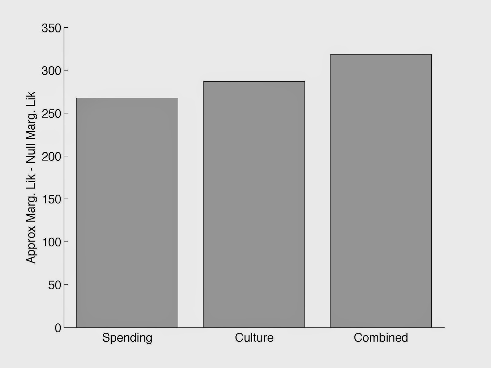
Everyone knows however that p-values suck. A better way to test whether both culture and spending have effects is to do model selection. That is, to see if a model including only culture, only spending or both is best at predicting the data we see. I calculated approximate values of the marginal likelihood of the data for all these 3 models - i.e. the probability of the data, based on each model. Comparing these to a simple null model that prizes are given at the same rate to all countries, we get the results below, again showing that including both effects gives a better prediction than either alone (marginal likelihoods shown in log values).

So surely now we can conclude that the Swedes are biased? Well conclude away...but be prepared to be wrong. Or right. Who knows? Because although this basic procedure (with a little more tweaking and a few more control variables) is ubiquitous in social science, where the observational study is king, it rarely tells us anything conclusively.

On the simplest level, there may well be an additional factor which we haven't controlled for that causes all these apparent effects. Maybe its really cultural distance to the USA that matters. Maybe (God forbid!) Sweden really does produce unusually excellent research. In estimating bias we often assume that fundamentally all nations, genders or whatever category are genuinely equal before any bias kicks in (for example in this previous post). This may be the enlightened thing to do, but it is certainly a strong assumption that we should be aware of.

But beyond these simple problems, there lie deeper issues. What we have just done is a case of Ecological Regression, which, though widely used, is essentially a precise codification of the Ecological Fallacy. For instance, if developing an academic culture, producing highly quality research and winning international science prizes tended to make a country more liberal, richer and more secular and self-expressive, then we'd see exactly the same results, without any need for a bias on the part of the ever fair and impartial Swedish Academy. 

So what can we conclude then? Generally, to be very cautious about over-interpreting correlations, or even significant regression coefficients after controlling for other factors. Causation is a slippery beast, and Ecological Regression won't pin it down for you, no matter how many stories the Daily Mail runs saying that X causes cancer. Is the Swedish Academy biased towards western scientists? I genuinely don't know, and this data won't tell me. I wouldn't be surprised if they were, any more than I'd be surprised if grant awarding agencies were biased in favour of men. But unless someone can do a double blind randomised test, you can continue believing whatever you like about the meritocratic value of our most prestigious prize.

This is a blog post I wrote about our seminar speaker at IFFS on Friday May 16, mainly for David Sumpter's blog and the IFFS website, but it won't do any harm to post it here as well. I and the speaker, Michael Osborne, did our PhDs together, and now he's one of Oxford's foremost experts on Machine Learning. In this presentation he described how Machine Learning will change everyone's employment in the coming century...

The future of automation

Depending on your perspective, technological development has been saving us from drudgery, or destroying our livelihoods, for centuries. From the very first domestication of animals we’ve been finding ways to perform tasks with less human action since civilisation began.

Last week Dr. Michael Osborne from the University of Oxford gave a presentation at the Institute for Futures Studies showing his predictions about which of us will be losing our jobs in the century to come. Michael, as an expert in Machine Learning, is interested in which jobs will be automated as a result of increasing artificial intelligence in the Big Data era. He and his colleagues have been impressed at the rapid pace with which tasks that were seen as impossible for computers to perform, such as driving a car or translating accurately between different languages have become almost routine.

Machine Learning itself can be used to predict which tasks are ripe for automation. First they gathered data on the skills necessary to perform over 700 different jobs, such as social sensitivity, manual dexterity and creativity. A panel of experts was then asked to predict which of 70 specific jobs would be automatable in the near future. Using Gaussian process regression, Michael and his colleagues learned a relationship between the skills a job requires and the probability that a computer will be able to perform, and extrapolated this relationship to the 700 jobs the panel had not evaluated. Their results give us a view on which sectors of the economy will be most affected by the continued rise of artificial intelligence. The graph below shows, by sector, what proportion of jobs are at low, medium or high risk of being automated. In general, those jobs requiring the most necessary social interactions and/or high level creativity appear to be safest from the coming tide of job losses, but none of us can rest too easy!

However, we shouldn’t be too distressed at this imminent redundancy. As Michael pointed out for example, while technological progress has reduced the workforce in agriculture from almost 40% of employment in 1900 to around 2% today, the total unemployment rate has barely changed. Technology has allowed society to move human labour to more productive areas. The results of Michael’s analysis also show that it is generally lower paid, lower skilled jobs that will be destroyed, giving hope that people will be able to move into better employment, if society provides them with the necessary skills.

Nonetheless, Michael also showed examples of resistance to change, such as the guilds of Tudor England blocking the development of machines for making textiles in fear of their members livelihoods. The ever increasing rate of automation, and the subsequent need for people to continually adapt to new careers and find new skills presents society with a powerful challenge, that may require new social contracts, such as a guaranteed citizen’s income and much more investment in public education to solve. It will be exciting to see where this process takes us!

Rethinking Retractions

This time last year I had to retract a paper I had recently published as a result of a coding error that invalidated the analysis. Now, one year later, a revised version on the same paper is about to be re-published, complete with an analysis of ALL THE DATA. Broadly speaking the results are the same as before, the methodology is still pretty novel, my career may just about have been salvaged from last years wreckage. With the whole episode (hopefully!) behind me, I wanted to write an article reflecting on the experience. While my view is obviously coloured by my own difficulties, I hope it will have some relevance to other scientists as well.

UPDATE: The relevant re-published paper is now available here

--------------------

Almost exactly one year ago I started this blog. I was also down in Australia, about to give a seminar entitled 'Prawns and Probability: Model Selection in Collective Behaviour'. The centre point of the presentation was going to be the work I had recently published on identifying interaction rules in groups of prawns. As the name of this blog suggests, it was also going to be the subject of one of the early posts here too. Having spent about 18 months on the research and writing before getting it published I was feeling pretty pleased with myself...

Back in the UK my friend and colleague from my PhD days, Michael Osborne, was also playing around with the prawn data, after I had passed it on to him as a nice example data set for him to test his numerical integration methods on. There was hope we might get a nice conference paper out of it. All was well with the world.

One night while I was finishing up my presentation slides I had a message from Mike come up on the computer. The conversation that followed is still starred in my gmail:

                    Michael: hey rich

11:45 

 Michael: it's going ok, I hope

  hey are you ready for some news

11:46 me: bring it

 Michael: dave reckons you only used 1/100th of the data in the .m files you sent us

  rather than 1/2 as it seems you intended

  basically just data from a single trial

 me: ...

  .........

  um, ok

11:47 what leads you/him to this conclusion?

 Michael: well, looking at the code

  our evidences approximately match yours on the 1/100th dataset

11:48 it's actually good news for us, because running on the whole dataset is crazy slow

  which allows us to make the argument that choosing samples is important

 me: ok, but how did i manage to only pull out 1/100th?

11:49 is it just 1:100:end?

  or are you only goijg on the evidences?

11:50 Michael: David: so there is something weird about the scripts we got

it seems like there is a bug that means that only 1/100th of the data is used
14:32
instead of 1/2 like they meant

me: ha

David: lines 12-15 of

logP_mc_...
14:33
so prawn_MC_results_script just hands it these cell arrays

and then it divides them in half 100 times

I think the code is supposed to just take every second row

but it takes every second cell, and does this over and over
----------------------------------------------------

In the 5 minutes it took to have that conversation my mood went from buoyant to despairing. Mike and his colleague David Duvenaud had found an error in the code I had used to analyse the data in our paper which had in a stroke invalidated all our results. This had a number of extremely unpleasant repercussions.

• I was now due to give an hour long seminar in ~3 days that focused on some completely false results.
• The paper I had been writing with Mike and David was now floundering without a data set, and my contribution had been wiped out
• The blog I had started had nowhere to go (hence the lack of posts over the last year!)
• Worst of all: I had to tell my co-authors on the original paper that our results were invalid, that we would have to retract the paper and that it was ALL MY FAULT for not checking the code well enough.

I won't bore you with the exact details of the next few weeks. Suffice to say I had a very drunk Skype conversation with my boss who was very good about the whole thing, I somehow gave a successful seminar despite having "CAUTION, POSSIBLY INVALID" over my most important results, and after crafting an extremely apologetic statement the paper was retracted. Mike and David found other data to play with. I wrote about some older topics in my blog. I didn't sleep very much for a few months.

The general unpleasantness of the whole experience led me to reflect on the nature of retractions and mistakes in the scientific literature. My conclusions:

• Mistakes like this must be relatively common. I may not be the most thorough person in the world, but I am far from the most careless. I made a similar mistake during my PhD but caught it shortly before publication (another few sleepless months there...). Any work that involves a lot of involved computational analysis of data by one or a few people must have a small but significant chance of including a coding error. Many of these doubtless have little impact on the results, but some will.
• My mistake was only caught because I gave my code to someone else. While this now makes it terrifying to do so every again, it also shows the value in journals insisting on code being made available. Given how involved some analysis of large data sets is becoming it is implausible to expect anyone to replicate your results without seeing your own code. The chances of peer-review catching this sort of error are somewhere between very small and non-existent.
• The business of retracting a paper is far too stigmatising. To be fair to PLoS, who published the paper, they were extremely good about the retraction and certainly didn't accuse me of anything underhand. Nonetheless, most peoples' first reaction on hearing I was retracting a paper was similar to Andrew King's: "Retracted? What did you do?" (actually, Andrew was very nice about it too, but his was the only reaction I had in writing!). Many other people gave me a there-but-for-the-grace-of-God-go-I look and said how awful it must be. Most of the stigma I felt came from the wider community who did not know me personally, but knew of websites like retraction watch, which, while aiming to shame fraudulent scientists also gives all retractions a a bad name.

Now I understand that retractions have often been associated with gross mispractice. Some successful scientists have been made a retract whole careers worth of publications after it was discovered they had been intentionally falsifying data. Of course this sort of thing needs to be stamped out as vigorously as possible.

BUT....

If mistakes are common (my assertion), and retracting a paper is awful (my experience), that seems like a recipe for encouraging cover ups and quietly ignored errors in the literature. I am not ashamed to say that the night I found out about my mistake I was initially tempted to ignore it. I'm glad now that I didn't, but a the time the little devil on my shoulder was trying to persuade me it wasn't worth the ensuing misery to correct an error in one paper among thousands, that the methodology was still sound, that it wasn't that big a deal. And therein lies the problem - a mistake in the literature seems like a small thing. In contrast, retracting a paper seems like a huge thing. Especially as it wiped from the record some of the work I was most proud of when my publication list was already a little sparse.

In conclusion, based on my experience I think there should be an easier, less painful and less stigmatising way to admit to serious but non-fraudulent errors in published work. The type of mistake I made will, I believe, only become more common. It doesn't mean everything the authors did was wrong, nor does it necessarily imply that there was any foul play. We should also advocate for making data and code publicly available alongside published work so more mistakes can be picked up before they have a chance to become accepted results. More should be done to create a system for distinguishing between mistakes and fraud.

Meanwhile, my advice to other scientists doing similar work to me is:

a) Don't trust the results in papers as being revealed truth just because they are peer-reviewed. 

b) I'm not going to tell you to 'do the right thing' if you find a mistake in your own (published) paper. Just be aware you might not be able to sleep until you do!

c) Go and check your code again now!

Please get in touch if you have had any similar experience, or if you disagree about anything I've written here. I'd be glad to know how people in the scientific community feel about these issues.

Follow up post - Rethinking Retractions: Rethought - details of everything that has happened since this post was first written

Pigeon Navigation (4): Identifying Landmarks

In this last post on pigeon navigation we'll see how we can identify the most important or "information rich" parts of a pigeons flight paths, and then equate these to the landmarks the pigeon uses.

Using the idea that a pigeon learns, and then attempts to follow a memorised `habitual route', we saw in the last post that we could use previously recorded flight paths to predict what future flights by the same pigeon, from the same release site would look like. We could assign a probability to any future path, thus deciding whether it was predictable or not after considering the past flights. The fact that paths typically became more predictable over successive flights was evidence that the pigeons were learning routes home and then sticking to them.

But how does a pigeon learn a route home. It is unlikely that it imagines a perfect line on the ground below it, representing some kind of idealised route it wants to follow. Memorising a complete continuous path, which has an infinite number of locations along it, is hard. Instead, the generally accepted hypothesis is that a pigeon learns its route by memorising a small number of landmarks which act as waypoints. This idea, known as `pilotage', supposes that the bird reaches one landmark, then reorients itself to head for the next until it reaches home.

Can we detect where these landmarks are, using the methodology we've developed so far? Of course we can!

Recall that we previously assumed that a flight path always consisted of 100 recorded positions, starting at the release point and ending at the home loft. We predicted future flights by using these 100 points on each flight path to estimate a habitual route  that the bird was trying to follow. We predict that future flights will also look like this habitual route, plus some variation that changes from flight to flight.

In principle we can choose to ignore some of this data. We can, if we want, choose to estimate the habitual path using only a subset of the data we have. For example, we might choose 10 random points of the 100 we have of each flight, then try to estimate the habitual route from these.

The first important point to understand for identifying landmarks is that such an approach will have varying degrees of success, depending on which points are selected. Consider the figure below

In each case the faint black line is the same simple bell curve. The black dots indicate 3 points on this curve that we are "allowed" to know in order to make a guess what the whole curve looks like. If we draw a smooth line through these three points we get the two red lines. Hopefully it should be clear that the red line on the left is a much better estimate of the bell curve than the very low red line on the right. Therefore, if I wanted to remember 3 points to try and remember the whole of the faint black line, I would better off choosing those on the left, rather than those on the left

But this is exactly what the pigeon has to do! It needs to remember a few landmarks so it can remember the whole of its route home. This suggests the second important point for identifying landmarks: the points that allow best estimation of the habitual route are the same points as the pigeon's landmarks. That means that we assume the pigeon does a good job of choosing the most efficient way to compress its habitual route into a few key points.

Since we can never measure exactly how well we have estimated the habitual route, we do the next best thing and test how well any set of possible landmarks allows us to predict future flights. If we call the subset of times that correspond to landmark locations at t__lm, and the full set of times as t__full, then our task is to choose t__lm to maximise p(x__n+1(t__full) | x_₁(t__lm), x_₂(t__lm), ..., x__n(t__lm))

And when we do this, we find landmarks that correspond to recognisable features of both the paths and the landscape beneath, such as below (remember I promised to explain what those red dots were...?)

The landmarks (the red dots) tend to be where the paths are very similar, since here the paths are a very good predictor of the habitual route, where the pigeon flies somewhere unexpected - the apex of the `C' shape - and where the path curves sharply. They also tend to be on the edge of forests and villages, above major roads and obvious features such as a church spire. 

[NB: Those with a machine learning background may see that this process is largely analogous to two other ideas. Active sampling, where we take data in an intelligent way to maximise our predictive power while minimising collection costs, and reduced rank Gaussian process approximations, where we use a subset of data points as `inducing points' to create a lower rank covariance matrix and speed up calculations.]

Pigeon Navigation (3): Habitual Routes

[NB: This post, and the rest of the pigeon posts will be quite mathsy. I've done my best to keep the maths as simple as possible - it should be possible to follow the argument without understanding all the working! On the other hand, if you do want to see the maths done properly, please read it properly formatted!]





Way back when this century was young, the navigation group in Oxford published a series of papers demonstrating that pigeons, when repeatedly released from the same site, would learn to follow the same route back the home loft each time.

If a pigeon is learning and following a route this ought to make its flight patterns predictable. If those flights are getting more and more predictable we should be able to observe that by using a model to predict the flights with increasing accuracy. In other words, we should have a model which gives the probability of a flight path, and that probability should get higher as our predictions get better.

In the last post we saw how to assign probabilities to individual flight paths using a Gaussian process (GP). The precise probability of a given flight path depended on the mean, m, and covariance, S, of that GP. I told you that the covariance dictated how likely the flight path was to be either smooth or wiggly, and we used the straight line between release point and home loft to create the mean. For convenience I'll write down the resulting probability as:

p(x| m, S) = GP(x; m, S)

Now, the reason we chose the straight line path to be the mean was that if we only look at a single path, and we have never seen this particular bird fly before, there is no reason to assume it will fly either one side or the other from this most efficient route. We don't expect the flight path to be perfectly straight, but we don't know beforehand in which direction it will go.

Imagine instead that we had already seen the flight paths below.

Now we should have a very good idea where the next path is going to be, somewhere close to the paths we have already seen. It looks like the pigeon is following a particular route home every time, so its unlikely to suddenly fly directly south from the release point next time. Obviously it doesn't fly exactly the same path every time, but each new flight path is like an imperfect attempt to fly some memorised route.

Lets imagine that we could look into the mind of the pigeon and retrieve exactly what its memorised route looks like. We can call this route h (for 'habitual'). Then we might replace the earlier straight line mean path with the one we now know the bird is trying to fly

p(x | h, S) = GP(x; h, S)


(I'm going to assume for simplicity that we know what  S is, but in practice we would infer it from the data)

Whats more, if we want to find the probability of several flight paths by the same bird, each an attempt to replicate h, we can simply multiply the probability of each path together, because each one is independent if we know h.

p(x₁, x₂, ...,x_n | h, S) = GP(x₁; h, S) x GP(x₂; h, S) x ... x GP(x_n; h, S)


Hang on! Surely those flight paths aren't really independent?! After all, they all look the same. Yes! But the reason they look the same is that they are all attempts to replicate h. They way each path varies around h is independent. All the shared structure in the paths is located in h.

Ok, thats nice, but the problem is that we don't know what h is. All we can see are a few paths that look a bit like h. But never fear - Bayes is here...we can use those flight paths we have actually seen to infer what h is. Recall Bayes' rule which allows use to reverse the order of the conditional probability:

p(h | x₁, x₂, ...,x_n, S) = p(x₁, x₂, ...,x_n| h, S) x p(h | S) / p(x₁, x₂, ...,x_n| S)


But we seem to be creating more trouble for ourselves. Now we need to know two more things, p(h | S) and p(x₁, x₂, ...,x_n | S). Are we digging a hole for ourselves?

No! The first of these terms is a prior distribution. It's how likely we think any particular habitual route would be before we see any real paths. So we need to place a probability distribution over a path that could lie anywhere between the release point and the home loft. Thats exactly what we learned how to do in the last post! Before we see any real paths theres no reason to expect the habitual path to be on either side of the straight line, so the probability of h is exactly like a single path on its own, with the straight line as a mean.

p(h | S) = GP(h; m, S)

The second term is the joint probability of the real paths, if we don't know what h is. This can be calculated by integrating over all possible values of h.


∫ p(x₁, x₂, ...,x_n | h, S) x p(h | S) dh


and this is where the theory of Gaussian processes really helps us. Integrals like this are really easy to do (using a few matrix rules...easy is a relative term!) when everything is Gaussian...


∫ p(x₁, x₂, ...,x_n | h, S) p(h | S) dh = ∫ GP(x₁; h, S) GP(x₂; h, S) GP(x_n; h, S) GP(h; m, S) dh


= GP ([x₁, x₂, ...,x_n], [m,m,...,m], Σ)


where those square brackets indicate that we're concatenating the n paths and n copies of the vector m. We have a big new covariance matrix, Σ, which is generated from S. If we want to mathematical details of how we do that I would suggest reading them in this paper (Open access), where it's all properly formatted without the restrictions of html. Here we'll just assume we know the matrix rules for multiplying Gaussian distributions together - check out Appendix A of my thesis if you're interested.

The upshot of all this is that we can calculate a probability distribution, p(h | x₁, x₂, ...,x_n, S), which tells us how likely any given habitual route h is, based on the flight paths we've already seen. Does it work? Well, look at the picture below, showing a set of flight paths from two birds, and the distribution (mean + variance) of the inferred habitual routes. The faint black lines are the flight paths, recorded from GPS. The thick black lines are the 'best guess' of the habitual routes, and the dashed red lines indicate how uncertain these are. The dashed black lines indicate where most future flight paths are expected to lie.

If we can infer what the habitual route is, we should then be able to do exactly what I suggested at the top of this post, and make some predictions about where future flight paths will be, and see if these become more accurate as the birds learn their routes. In fact, we have already done everything we need. We calculated the joint probability of n paths, assuming that we didn't know the habitual route.

 p(x₁, x₂, ...,x_n| S) = GP ([x₁, x₂, ...,x_n], [m,m,...,m], Sigma)

if we want to calculate how probable path x_n is, based on the previous n-1 paths, we simply calculate the joint probability of x₁, x₂, ...,x_nand of x₁, x₂, ...,x_n-1

p(x_n | x₁, x₂, ...,x_n-1| S ) = p(x₁, x₂, ...,x_n | S) / p(x₁, x₂, ...,x_n-1 | S)

So lets test it out. In the experiments done in Oxford the typical procedure was to release the same bird 20 times from the same spot. What happens if we calculate how likely each of these flight paths are, based on the previous 2 flights immediately before?

That graph shows the (log) probability of the next path becoming higher over time - the pigeons are becoming more predictable, just as we hoped! Where the y-axis is equal to zero is the point at which the paths are more predictable than if we just guessed wildly without seeing any other previous flights. Therefore we can say that after ~10 flights the birds are more predictable than random - they have learnt their routes. 

This demonstration of increasing predictability is a nice alternative way of seeing route learning that was previously shown by measuring the average distance between successive paths, but its not immediately clear why it should be any more useful. In the next post we'll see how we can see now only that the route is being learnt, but where it is being learnt, to identify where the landmarks the pigeons use to navigate are and what they might be. 

Pigeon Navigation (2): GPs and GPS

In the last post I introduced the idea of using Gaussian processes (GPs) as a tool for modeling homing pigeon flight paths. In this post I'll give a few more details of exactly what this entails.

For our purposes a pigeon flight path consists of a number of recorded 'x' and 'y' co-ordinates from a Global Positioning Satellite (GPS, don't confuse the two!) recorder, each with a time stamp 't'.

For the sake of simplicity, lets imagine that any such path begins at time t=1, and ends at time t=100, with 100 recorded points equally spaced in time between (this isn't strictly true, but it won't make any real difference in understanding this). How can we assign a probability to this path?

What we do is claim that the 100 recorded 'x' co-ordinates are a sample from a 100-dimensional multivariate Normal distribution, N, with some mean vector, m and covariance matrix S.

p([x₁, x₂, ..., x₁₀₀]) =  N([x₁, x₂, ..., x₁₀₀]; m, S)


(NB: the 'y' co-ordinates will have their own distribution, but we can get away with just considering the 'x's for now, we'll worry about the 'y's a bit later )

Now, a 100-dimensional distribution sounds a lot scarier than it actually is. All this is telling us is that these 100 recorded locations are connected, e.g. x₆is likely to be very close to x₅, since the pigeon does not have time to move very far between t=5 and t=6. Conversely, the connection between x₅ and x₉₀ will be much weaker, since the bird is free to move a large distance during that time. The Normal distribution provides a convenient tool for assigning probabilities to large numbers of correlated variables, and its mathematically easy to deal with (as we'll see as we go further).

So what are m and S? The mean vector, m, is quite simple. It is where we "expect" the bird to be at a given time. Since we know where the bird starts and finishes, we can expect that x₁ will be at the release point and x₁₀₀ will be at the home loft. Without any other information it is reasonable to assume that the other 98 points should be spaced equally along the straight line between the release point and home. Of course, they almost certainly won't actually be exactly on this line, but there is no reason for us to believe the bird will show a preference to fly one way or another before we see any data. In the picture below the thick black line indicates the locations of m

The covariance matrix, S, specifies two things. Firstly, the diagonal entries, such as S_ii, specify how much the values of x_i are likely to differ from the expected values of the mean, m_i. The other entries, S_ij, indicate how strongly connected the values of x_i and x_j are. High values of S_ij mean that x_i and x_j will be strongly correlated. If S_ij is zero then there is no correlation between x_i and x_j.

We don't want to have to specify a correlation between every pair of points individually. Instead we construct the matrix S using a covariance function k(i, j), which depends on the difference between i and j, e.g.


S_ij = k(i, j) = k₀ exp(-(i-j)^2/L)

with this function the correlation between x_i and x_j gets weaker as the difference |(i-j)| gets larger. The parameter L determines how quickly this happens. If L is large then correlations will persist over longer separations between points. If L is very small then correlations will almost disappear after just few time steps. If the correlations between points persist for long periods of time then the path will be very smooth, since any points close to each other in time must also be close in space. Equally, if L is small then the path can be much more 'wiggly' and the bird can change its position quickly. k₀ tells us how uncertain the path is. If k₀were to be zero then all of the entries of S would be zero and the path would be forced to lie along the mean - their would be no uncertainty. Large values of k₀mean that any path can be quite far from the straight line. The plot below shows k(i, j) as a function of dt = |i-j|, using different values of L (the Input Scale), with k₀set to 1.

By applying the function k(i, j) to every pair of points we can construct the full matrix S, which will typically look like the example below:

The values of S peak along the main diagonal and decay as you move away from this. The width of the central red band shows how strongly correlations persist over time. Here points are correlated when they are within about 20-30 time steps of each other. 

So, we can get the probability of any path of 100 points, given only a mean and a covariance matrix. The mean, as we saw, is specified simply by knowing where the bird starts and finishes. The covariance matrix is specified by only 2 parameters, k₀and L. So, the probability of the x co-ordinates depends only on these two parameters (as well as knowing the start and finish, which we'll assume are always known)

p(x | k₀, L) = N(x; m, S(k₀, L) )

We can take this further and either find the optimal values of k_0 and L, or even better, sum over our uncertainty by using an appropriate prior distribution that expresses how likely we think different values of these parameters are (see the post on Bayesianism for more details). This gives us a probability for the path, independent of any particular choice of parameters.

p(x) = ∫ ∫  p(x | k₀, L)p(k₀)p(L) dk₀ dL = ∫ ∫  N(x; m, S(k₀, L) ) p(k₀)p(L) dk₀ dL

Now, remember those y co-ordinates we removed? We can apply exactly the same analysis as we've done here for the x co-ordinates, but for the y co-ordinates instead, with their own mean (derived again from the straight line path) and covariance (the bird may vary more along x or y axes). Not knowing anything in advance about how the bird's path will vary around the straight line we can treat the x and y co-ordinates as independent (once the mean path is accounted for). Therefore we can get the probability of the whole path simply by multiplying the two probabilities for both sets of co-ordinates.

p(path) = p(x)p(y)

So thats how we go about assigning a probability to a path. This probability will reflect our instincts about how 'likely' a path is: paths that lie close to the straight line will be more likely than ones that go off in some bizarre direction, and paths that are excessively 'wiggly' will have a low probability. Nice smooth flight paths in the vague vicinity of the straight line are what we expect a flying animal that cares about energy efficiency to produce.

This might all seem a little dry and you may be wondering exactly what we gain by doing this. For now, I'm going to have ask you to trust me. In the next few posts we'll see how the simple act of matching paths to probabilities gives us some exciting analytical power.

Pigeon Navigation (1): Paths and Probability

How do birds navigate successfully over huge distances from temperate to tropical regions and back every year? How do homing pigeons know how to get back to their owner's loft quickly enough to win a race? Is there some way to control the number of pigeons in Trafalgar Square [or insert your country's pigeon hotspot]?

All good questions. None of which really interest me.

How can we mash up the science of pigeon navigation and a bit of probability theory and come up with something fun and faintly ridiculous? Now you're talking...

For a bit over 10 years now researchers having been attaching GPS devices to the backs of domestic homing pigeons (Columba livia to our classicist friends) before releasing them in more or less odd places. If and when these pigeons make it home, the devices can be removed and we can see exactly where the pigeon has been in the interim (typically at a resolution of a couple of metres, once every second).

This is what a pigeon looks like. Thats a GPS tracker on its back.

A few pigeon paths recorded in the Oxford area. Those red dots sure look exciting don't they? We'll be getting to them eventually...

With such data, our intrepid scientists have shown that probably use landmarks, learn routes home, seem to follow roads and often co-operate in getting home. Sadly, while these findings have revolutionised a popular field of study, been hugely cited and generally proved more than averagely seminal, they didn't include very much probability theory, so I'm going to go ahead and pretty much ignore them from here in.

But where there's data, there's chance to get some machine learning going. So let's get to it...

Paths and Probability


There are many things we might want to learn from the recorded data from the GPS devices. In my research I try to frame learning as a test of various hypotheses using data to adjudicate between them. For example, if we want to learn whether pigeons genuinely follow idiosyncratic routes (which we will) we need to know if the data is more or less likely given this hypothesis than the alternative. If we want to know if the pigeon uses landmarks, we need to find a way to say if the GPS data is more or less likely based on some hypothetical set of landmarks the bird might be using. We need to use probability theory as a link between our data and our theories.

The many recorded locations that a pigeon visits constitute elements of a path that the pigeon actually flies. As with anything probabilistic, we need to start off by finding a way to ask how likely the data (the recorded positions) are. How probable is it that the pigeon flew this path, rather than some alternative route? How can we place probabilities on observations of flight paths?

Well, lets try and get there one step at a time. First I'll just try to give you some idea of the approach we're going to take. In subsequent posts I'll flesh this out with some actual maths.

 If I asked you to place a probability on where the middle of the path (say, the 50th of 100 locations) would be, how would you do it? A reasonable guess would be that on average it would be half way between the release point and the loft. But as the picture above shows, its likely to vary around that point quite a bit. Wherever you think its going to be, you can specify this as a probability distribution, a Gaussian (Normal) distribution, centred on where you think it will be and with a standard deviation that represents your uncertainty.

Now imagine I ask you to put a similar probability on the locations 1/3rd and 2/3rds of the way along the path. We could just as easily make a guess and place Gaussian distributions at both of the points to represent where we think the bird will be. Likely these will be directly 1/3rd and 2/3rds of the way between release and loft. But look at that picture above. If the pigeon starts out to the left of the straight line, its likely to stay out to the left later. So our two locations are going to be correlated, if one is left of centre, the other is likely to be too. They have a joint probability distribution.

The pictures below give some indication how this joint distribution works. We have two correlated variables. Initially we are quite uncertain about both (A). Then we measure one, reducing its uncertainty to zero (B). In addition, the uncertainty in the second variable is reduced, and the expected value moves closer to the first measured value.

(A) Two correlated, unmeasured variables

(B) Variable 1 is measured, variable two is less uncertain

Now, we can extend this to lots of different locations along the path. It is reasonable to imagine that locations will be more correlated the closer they lie along the path. Lets assume we can state a function which we call the covariance function, k(t1, t2), which states how strongly two values (t1, x1) and (t2, x2) should be correlated, and that this gets weaker as the separation of t1 and t2,  dt = |t1-t2| becomes bigger, such as the functions in the figure below.

Correlations get weaker as the difference in t values increases. How fast the correlations decrease depends on the covariance function, k(dt).

Making that assumption, and looking  at 10 points, all jointly distributed, we might get figures like those below

(A) 10 unmeasured variables, correlated according to separation

(B) Measure some variables, others become less uncertain in response.

Going one step further, we might take the number of points we are interested in to infinity, for a continuous path, and then measure just a few of those points

A continuous range of variables, measured in 3 places

What we're getting too, through this exercise, is the concept of a Gaussian process, which is a probability distribution over continuous paths or functions. Much like the Gaussian distribution gives a probability of seeing any number, or set of numbers, a Gaussian process (GP) gives the probability of seeing any path, or any set of points measured on that path. The standard Gaussian distribution can describe any finite number of jointly distributed variables, the GP is simply a Gaussian distribution with an infinite number of variables, representing every possible point on the path.

Gaussian: P(x) = N(x; mean, variance)

Gaussian process: P(path) = GP(path; mean path, covariance function)


The most important property of a GP is that any subset of points on the path (such as the recorded positions from the GPS device - don't confuse GPs and GPS!) follow a multivariate Gaussian distribution,

P(recorded positions) = N(recorded positions, mean positions, covariance matrix)


We'll discuss more about exactly what the covariance matrix and mean positions represent in the next post.

Great! We're on our way. If we can assign probabilities to paths in a consistent manner we can ask if observed paths are more or less likely based on different hypotheses, which allows us to use data to select between those hypotheses. In the next post I'll give a rundown of the properties of GPs and how they work.

[In a switch of textbook, for these pigeon navigation posts I'll be advising you to look at the definitive guide to GPs, Gaussian Processes for Machine Learning, by Rasmussen and Williams, and what I have to assume is the definitive work on using GPs to analyse pigeon flight paths, Prediction of Homing Pigeon Flight Paths using Gaussian Processes, by one R. P. Mann]