How Fish Shoal (5): Separating Different Effects

In this final post on the analysis in our paper on fish shoaling, I'll show how we can adapt the technique of fitting a function using a neural network, using this to isolate the various different cues that the fish respond to simultaneously.

In general we might imagine that a fish moving in a shoal is presented with an array of potential stimuli at any moment. Just for starters, it has the positions, movements and behaviours of its many neighbouring fish to consider. In addition to this there are other environmental cues, such as the positions of the walls of the fish tank in a laboratory experiment, or the possible locations of predators in the wild. We can expect that the behaviour of the focal fish at any moment will be due to a combination of all these effects (I'm intentionally avoiding the words 'sum' or 'product' for reasons that we'll soon see).

Now, in the last post we learned how we can fit the behaviour of a focal fish as a function of any input stimuli that we choose. We saw an example using just the position of the nearest neighbour to predict the acceleration response of the focal fish. There is nothing in that approach to stop us instead using far more input stimuli. We could, for example, construct a neural network to predict the acceleration from the positions of the nearest 3 neighbours.

This would, in principle, allow us to learn how the acceleration of the focal fish depends, in potentially very complex ways, on the positions of its 3 nearest neighbours (NNs - don't get confused with neural networks!). However, such an approach has a few significant drawbacks. Firstly, from a technical viewpoint, the larger we make the space of possible inputs (i.e. the more stimuli we use), the harder it becomes to train the neural network. The more inputs we have the more combinations of those inputs that are possible. It becomes less and less likely that our data will cover a large enough proportion of those possible combinations to allow us to learn the connections between inputs and outputs.

Secondly, even if we could learn a function of the 3 positions (6 variables in total, each position being an angle and distance), how are we to 'see' what we have learnt? We may be able to try new combinations of the inputs and find the predicted acceleration, but it is going to be almost impossible for us to visualise the function.

Finally, how can we relate this back to previously established theories of collective motion? If we learn some highly complex function of the positions of all the neighbouring fish, what does that tell us about the simple rules of interaction that have previously been the standard way of understanding these phenomena?

We can get around these difficulties by considering the sort of interaction rules that have been suggested before. These have almost exclusively considered additive responses - the response of the fish to 2 neighbours is simply the sum of the response to each neighbour individually. This is akin to most effects in physics - the force on a spaceship is the sum of the gravitational force from the Earth and the gravitational force from the Moon, and the gravitational force from the Sun...etc. The existence of the Moon doesn't change the force exerted on the spaceship by the Earth (at a specific moment in time).

So we can propose a model where the acceleration of the focal fish is a function, f, of the positions of 3 neighbours (p₁, p₂, p₃), this function itself being the sum (see why we avoided that word earlier) of 3 simpler functions, g₁, g₂, g₃.

Acceleration = f(p₁, p₂, p₃) = g₁(p₁) + g₂(p₂) + g₃(p₃) + residual

Now, just as we can model a function using a neural network, we can model 3 functions using 3 neural networks. The eventual acceleration is now the sum of the outputs from those 3 networks. I'm going to stop drawing each network properly and just treat them as black boxes, as I encouraged you to do in the last post.

So the task of estimating one complicated function by learning one big neural network is now changed to the task of estimating 3 hopefully simpler functions using 3 smaller networks. The question is how to learn all 3. There is a choice to be made - do you try and learn all 3 simultaneously, or do you prioritise some over others.

In our paper we took both approaches for different subsets of the stimuli. We considered the position of the 3 nearest neighbours, but also the past behaviour of the focal fish and the position of the wall, give us a schematic as below.

Or, in equation form:

Acceleration = g_past(past) + g_wall(wall) + g₁(p₁) + g₂(p₂) + g₃(p₃) + residual

We made two biologically motivated reasonings to decide how to approach learning this combination:

1. There is no reason to suspect, a priori, that the past behaviour of the fish, the position of the tank wall or the positions of the neighbouring fish are more or less important than each other

2. It is implausible to imagine that the focal fish interacts with its 2nd or 3rd nearest neighbours but not with the first nearest. 

Therefore we will learn the first three networks (past, wall, NN1) simultaneously, since each of these should have the chance to be the primary factor in predicting acceleration. Networks 4 and 5 (NN2 and NN3) will be learned subsequently, using whatever part of the fishes' acceleration that has not been accurately predicted by the first 3 networks. This means, for instance, that the interaction between a fish and its second nearest neighbour will only be allowed to account for what cannot be predicted by its interaction with its second nearest neighbour.

The process of learning multiple networks, either simultaneously or in succession is relatively similar. We iteratively learn each network, while assuming that the others are already known. Lets look at how we learn the networks associated with the past, the wall and the nearest neighbour:

1. Start each network in a random configuration, just like when we learn a single network.

2. Now, we assume that the networks associated with the past and the wall are known and correct. We pass our measured values for these stimuli into the networks and record the output, getting a predicted acceleration_past+wall (recall the USE function on the black box from the last post)

3. We now learn the nearest neighbour network using our measured values of the nearest neighbour position as inputs, and the difference between the actual acceleration and the predicted acceleration as outputs

4. Once the NN1 network is learnt, we fix its state and then apply the same technique to learn the past network. Fixing the wall and NN1 networks in their current states we predict what the acceleration should be from the wall and nearest neighbour alone

5. Then, like in step 3, we now learn the past network, using the difference between the predicted and observed accelerations as the output

6. Having learnt the past network, we fix its new state, and we predict the acceleration from the past and the nearest neighbour networks

7. And now we learn the wall network, using the measured values of the wall position and the difference between the predicted acceleration and the observed acceleration

8. We can now test how good our 3 networks combined are at predicting the real acceleration by feeding the measured stimuli through all 3 in their current states.

9. Now we have learnt each of the first 3 networks once. However, we are not finished. From this point we go back to stage 2 and go through stages 2 to 8 again, repeating the whole process until the error between predicted acceleration and real acceleration stops improving.

So by this process we have learnt, simultaneously, the functions associated with the past, the wall and the nearest neighbour. The process of learning each network in this iterative fashion divides the observed accelerations into components associated with the different stimuli in a way that creates the best match between the measured values, assuming that the additive assumption is correct. It is of course possible that there are more complicated interactions that depend on, for example, the positon of the wall and the nearest neighbour in some complex non-additive fashion. We have found the best additive function that estimates the true process.

Now, having found these three networks, we are in position to successively learn the interactions with the second and third neighbours. Remember that we do these after the first 3 since it is hard to imagine a fish consistently ignoring its nearest neighbour while attending to its second nearest neighbour. As such we only learn each of these once, rather than iterating.

10. Group all 3 of the networks we learned before and predict the acceleration

11. Now learn the second nearest neighbour network (NN2) based on the difference between this prediction and the observed acceleration

12. Now group all 4 of the networks we have learnt so far and predict the acceleration

13. Learn the 3rd nearest neighbour network based on the difference between these predictions and the observed accelerations

14. Phew! Now we have finally learnt every network. We can make predictions based on all 5 networks to test how well the combination predicts the real accelerations

15. But nicely, since each network has only 1 or 2 inputs, we can also input the range of possible values for each input into its respective network and plot the output, enabling us to visualise each component and solving our earlier problem with visualising a high dimensional function. When we do so, we get something that looks a lot like the figure below. The results from the past network are not shown, only those from the wall and the 3 neighbours (from top to bottom respectively). On the left hand side we have the predicted accelerations from each of these networks. On the right hand side we also have the predicted turning angle, using the same process but with measured turning angles instead of accelerations. Recall that each plot is a semicircle because the funtions are assumed to be symmetric (acceleration) or anti-symmetric (turning angle)

As we saw in the last post, the interaction with the nearest neighbour replicates many of the features we expect, including distance dependent repulsion and attraction between the two fish. The other interesting result here is how little structure there is for the functions associated with the second and third nearest neighbours. In our paper we interpret this as evidence that the fish primarily interact with their first neighbour only. Such a strong biological interpretation comes with necessary mathematical caveats. It is important to be clear that we have only learnt the best function for mapping stimuli to behaviour out of those which fit the additive structure we proposed. As shown in a another paper published alongside ours, interactions may not always be additive. Also, technically what we have shown is that the positions of the second and third neighbours do not help us to predict the behaviour once we known the position of the first nearest neighbour. While this suggests that no interaction takes place these are subtly different statements.

Despite those final caveats, learning combined functions in this manner is a powerful tool for separating effects in the data, and for learning patterns that may be obscured by other unknown factors (such as the response to the walls of the tank here). I hope you find this useful when considering your own data!

If you want to know about this sort of technique in more detail I can suggest starting on the Wikipedia page for Expectation-Maximisation, or let me plug again (unpaid and unrequested!) my suggested text: David Mackay's textbook, Information Theory, Inference and Learning Algorithms (free online).

How Fish Shoal (4): Using a Neural Network to Learn From Data

To recap, in the first post on this topic, I started by asking how we can use recorded data of fish movements in groups to learn how they interact. I stated that we can see this as inferring a function between the environment and the fish's behaviour, and in the subsequent posts we looked at how we might estimate functions using regression, arriving at the idea of a neural network as a highly flexible tool for performing non-linear regression. In this post we'll see how we can practically use neural networks (as one possible tool among many alternatives) to learn from data, and how this is actually coded in Matlab to show how few of the details we need to concern ourselves with to start doing useful inference.

I'll be referring to code that utilises the Netlab toolbox in Matlab, which you can download for free, and which you can install simply by unzipping the downloaded file and adding the directory to your Matlab path. The code I will use is specific to Netlab, but the basic method applies to using any similar toolbox.

Inference always begins by deciding which outputs (behaviours) we want to predict from which inputs (stimuli, environment). The recorded positions of the various fish over time taken from video tracking are only useful once we make this assignment. In the case of our research we looked at the relative positions and directions of each fish's neighbours in the group as the inputs, and the fish's responses of accelerations (or deceleration) and turning angle, as shown in the figure below taken from our paper.

The relative position and direction of a neighbour (yellow) from the focal fish (red)

So first we take all the recorded positions of the fish, and for every fish at every time step we calculate the following quantities:

1. The angle (theta) and distance (r) to the nearest neighbour, the second nearest neighbour, third nearest etc.

2. The direction (phi) of each neighbour relative to the focal fish

3. How much the fish accelerated (a) and turned (alpha) on the next time step

We also measure quantities associated with where the wall of the tank is relative to the fish, but I'll ignore these for now. 1 and 2 here are our inputs, the stimuli. 3 is the behaviours - what the fish did next in response to the stimuli.

So, assuming that we've tracked our fish and measured the above, lets get inferring....

Let's try seeing how the acceleration of the focal fish is related to the position of the nearest neighbour. Once you've got Netlab installed, you can build a neural network in just one line

my_nn = mlp(2, 10, 1, 'linear');


my_nn: is your neural network (remember from the last post, it can also be called a Multi-Layer Peceptron - mlp)

2: is the number of inputs we want to use. We will be using the angle and distance to the neighbour.

10: is the number of 'hidden nodes' - thats the number of nodes in the middle layer of the diagram we saw in the last post. We can change this number - more nodes make the network more flexible but harder to learn well. I find 20 tends to work ok, but always experiment! Each node will be a sigmoidal function of the inputs, but we're not going to worry about these details here.

'linear': means that the output will be a weighted sum of all the hidden nodes. The only real reason to change this is if the outputs are binary rather than continuous.

Now you have a neural network! But at the moment is doesn't do very much. It's been configured in a random state. You can try putting some numbers in and seeing what come out using mlpfwd


y = mlpfwd(my_nn, [x1, x2]);


where x1and x2 are any possible values of the angle and distance to the nearest fish you want to try, and y is the predicted acceleration. At the moment those predictions will be meaningless, as the network hasn't learnt anything.

Now comes the useful bit. Assume we have three vectors containing the data, theta is a vector of angles to the nearest fish, r is a vector of the distances to the nearest fish and a is a vector of how much the fish accelerated. Make sure these are column vectors. Then we can train network using just a few more lines of code.

options = zeros(1, 18); options(1)=1; options(14) = 100;
my_nn = netopt(my_nn, options, [theta, r], a, 'scg');


netopt is a function that trains the network, based on the data its given. It tries to find the values for all the parameters (like the 'slopes' in the last post) which will produce the best match between what actually comes out of the network when we put the inputs (position of the nearest neighbour) in, and the behaviours we tell it should come out (i.e. the measured accelerations). options is, as the name suggests a number of possible options. Here we only use 2. The first tells Matlab to show the error values as the algorithm learns, the 14th tells netopt to run 100 iterations of the learning algorithm. The learning algorithm is something called 'scaled conjugate gradients', which is the 'scg' at the end.

Now we can input any values of theta and r to the network and it should output a value of the expected acceleration that fits with the data it has already seen. That is about 90% of everything you need to know to start doing inference with a neural network today. All the diagrams and equations in the last post are nice to have in the back of your head while doing this, but essentially you can treat the neural network as a black box. You put data in, in the form of known inputs and outputs. You press a button to make the network 'learn', and then the box will tell you what output you should expect for any input you offer it.

First we show the network some known examples

..then we ask it to predict the output for other inputs

This is in fact the basis of pretty much all of machine-learning. Take a number of known examples of something, such as images of handwritten letters. Plug them into a learning algorithm (of which a neural network is but one among many) to train it. Then use the same algorithm to predict what some unknown examples are.

Now all that remains is to try inputting all the possible values of theta and r that we might be interested in. In our paper we made the further simplification that the function would be symmetric around the axis of the fish - i.e. if the fish will accelerate when a neighbour is ahead on the left, it will also do so if the neighbour is ahead on the right. So we test values of r between 0 and some maximum (like 40cm), and angles between 0 and pi (everywhere on the left of the fish). In Matlab we can make vectors of these test inputs like this:

r_test = linspace(0, 40, 100);
theta_test = linspace(0, pi, 100); %this gives us 100 values of each input


[r_grid, theta_grid] = ndgrid(r_test, theta_test); 
test_input = [r_grid(:), theta_grid(:)];
%this matches every value of r to every value of theta so we can test all pairs


test_acc = mlpfwd(my_nn, test_input); %this puts our test inputs through the network we learned


test_acc = reshape(test_acc, size(r_grid)); 
%and this makes the output accelerations into a matrix so we can visualise it

X = cos(theta_test)*r_test';

Y = sin(theta_test)*r_test';

pcolor(X, Y, test_acc);

%This visualises the output on a nice semi-circle

And so finally we get a plot showing what the network thinks the fish will do for any given position of the nearest neighbouring fish

That B is because this comes from a multipanel image, as we'll see soon

So we confirm some previously held beliefs about how interactions like this work. The focal fish accelerates to catch up with a neighbour in front. It slows down to rejoin a neighbour behind. And if a neighbour is too close (near the centre), this is reversed to move the focal fish to a more comfortable distance.

So in a few lines of code by us, and a lot of preprogrammed code by the makers of Netlab, we have done some quite sophisticated inference with a minimum of real maths. Of course, there are some complications in now getting from the 90% you already know to the 100% you need to get publication ready. You'll need to concern yourself things like multiple local minima of the squared error, cross-validation and such other things. But these are things to worry about once you've got your hands a little dirty and started actually doing some inference...none of them mean you can't start applying these techniques to your data TODAY!

In the next and probably last post on this topic I'll show how we go from learning this relatively simple function with just 2 inputs, to a more complex function accounting for the positions of many neighbours, and we'll investigate the perils of correlation and confounding.

[Again, if you want to read more about the details of any of these techniques, I recommend David Mackay's textbook, Information Theory, Inference and Learning Algorithms (free online). Netlab also contains a large number of demo scripts, of which demomlp1.m demo is similar to this post]

How Fish Shoal (3): From Linear Fits to Neural Networks

In the last post we looked at how we could adjust the slope of a simple straight line fit to minimise the residual error between the data and the approximating function

Behaviour = Slope x Stimulus + residual

Although linear regression like this can be very powerful, and is often used to determine if two variables are linked (via correlation analysis), in general we cannot expect that animal behaviour is always so straightforwardly related to the stimuli or environmental cues we are interested in.

Consider for example how good you might feel over the course of an evening of heavy drinking. Here we can quantify the 'stimulus' as the number of drinks you consume. While some people are lucky enough to always consume in moderation to their acceptable intake, I would wager you have encountered evenings where your general state of enjoyment follows a trend like the one below.

Enjoy inference responsibly...

How can we fit a function to a more complicated looking curve like this? One solution would be to try and guess the shape of the curve....but what function does it look like? If we choose badly then we'll never get a good fit to the data.

We'd like a more flexible alternative that doesn't require so much guesswork. To see how we can get there, first we need to understand how we might apply the previous straight line fitting techniques when we have multiple stimuli. Imagine we think that an animals behaviour is a function of two stimuli

Behaviour = f(Stimulus₁, Stimulus₂)

Well, how about starting by extending the equation we had for a straight line. The original equation for just one stimulus was:

Behaviour = Slope x Stimulus + residual

For reasons that will become clear, we can draw this relationship using the following schematic

Extending this to two stimuli we have two slopes:

Behaviour = Slope₁ x Stimulus₁ + Slope₂ x Stimulus₂ + residual

and similarly a new picture, showing that the behaviour comes from adding the two different factors:

Now the behaviour varies in response to both stimuli. Each slope tells us how strong the relationship between stimulus and behaviour is, and we can find out what these slopes are in much the same way as before, either by trying different values until we get the lowest squared-sum-of-errors (see the last post), or by using the special formulae that exist for telling us the best solution. I don't intend to worry about these formulae here, but if you want to find them or see where they come from then the Wikipedia page on Ordinary Least Squares is a good place to look.

We can extend this basic approach further, including more and more stimuli. But, at this point you may be wondering "How does this help us fit functions like the one about drinking enjoyment above?" At this point we employ a wonderful little trick. Remember we talked about guessing the form of that function? I said that this would be too restrictive. But what if we guess lots of functions? 

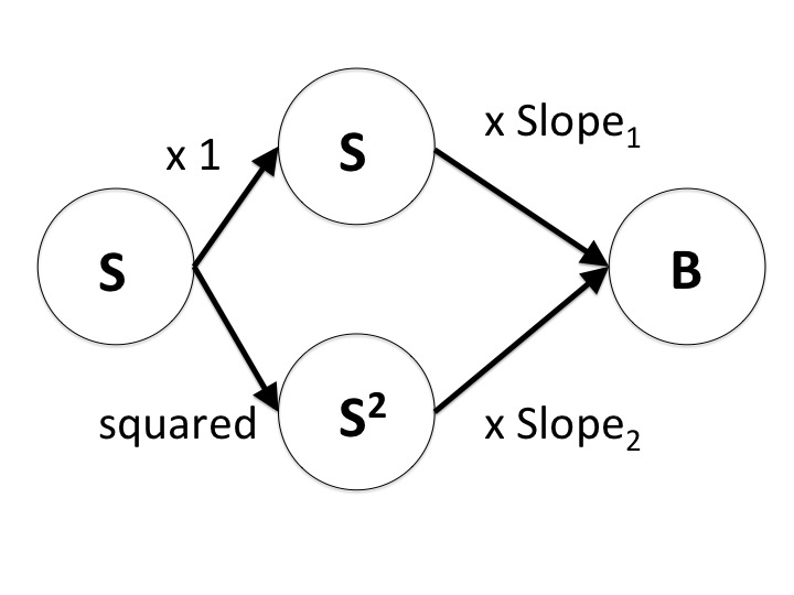
The trick here can be seen simply by taking the equation for two stimuli we had above, but now imagine that stimulus 2 is related to stimulus 1. Instead of two different stimuli, imagine instead that we replace stimulus 2 with a function of stimulus 1. Lets try something simple, like Stimulus₁².

Behaviour = Slope₁ x Stimulus₁ + Slope₂ x Stimulus₁² + residual

Now, if we find the best fit values for these slopes, based on the observed values of Stimulus1 and Stimulus₁² we are actually fitting a non-linear, quadratic function to the data. If we know what Stimulus₁is then we can easily calculate Stimulus1^2, and then we can treat them as if they were different stimuli. Fitting this function is still the same process as before - we choose different values for the slopes and find those that produce the lowest residual errors. See that our schematic of the model now has an additional layer between the stimulus and the behaviour.

We can take this simple trick further. Instead of many stimuli, we can use many different functions of the same stimulus.  Consider a set of different functions of the stimulus, g_i(stimulus), where each value of i specifies a different function. We can model the behaviour as being a sum of these functions, each with its own slope

Behaviour = Slope₁ x g₁ (Stimulus) + Slope₂ x g₂ (Stimulus) + Slope₃ x g₃ (Stimulus)... etc

These functions could each be different powers of Stimulus, giving us a polynomial fit, or they could be any other set of functions. The key point here is that instead of guessing one kind of function to fit, we can try lots of different functions and weight them according to how important they are. Just as in every case before, when we try different values for the slopes, we get different residual errors, and we aim to find the best values that minimise those errors. Of course, as the number of slopes increases it becomes harder to find the best values easily, but in principle the task is the same.

The schematic of this kind of model (below) shows that we now have an expanding middle layer, where each circle represents a different function of the stimulus. The value of Stimulus is passed to each of these functions. The output of each function is then weighted according to the value of its Slope and passed to the Behaviour, which is made from the sum of all these bits.

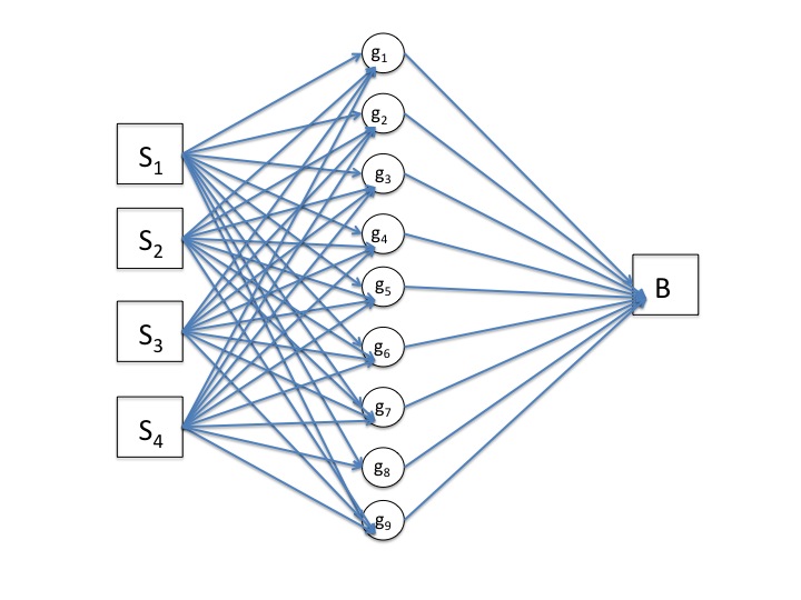
The next and final stage is to consider developing this middle layer one step further, so we can once again consider multiple different stimuli. Instead of just one stimulus at the start which leads to our middle layer, imagine we have many stimuli to consider. Each function in the middle layer is now dependent on all the different stimuli, so e.g. g₁ = g₁ (S₁ , S₂ , S₃ ...). Connect each stimulus to every function in the middle layer...

Don't worry about the switch from circles to squares or from black arrows to blue, I'm just reusing an old image!

Now we have a model which is going to look very complicated if we write it down as an equation. In essence though the idea remains the same as our first linear model. Along each line we simply multiply the input by some number, just like the slope of the linear plot. The behaviour predicted by the model is given by adding up all the different bits coming out of the middle layer into the final node, and we can adjust the multiplying numbers on each line to get the lowest error possible. When we find the best values for these numbers we have something which acts as a function taking stimuli to behaviour. We can then put it any value of stimuli we are interested in and see what the function predicts the animal will do.

You may have seen something like the above picture before. It is an example of what is known as an artificial neural network and is of a special type called a multi-layer perceptron. In such models the functions in the middle layer are usually sigmoidal functions that aim to mimic the highly thresholded response of real neurons to stimuli in the brain. Each function takes in a weighted sum of the stimuli, S, and sends out an output according to a profile like that below.

These neural networks provide us with a tool which can fit extremely variable non-linear functions of many stimuli. Neural networks have a lot of parameters that can be varied, each one essentially like the slopes we learnt for the linear model. Just as before, when these parameters are changed they alter the residual error between the behaviour predicted by the model and the observed behaviour. Unfortunately there is no general solution that quickly tells us what these parameters should be like there was for the linear model, but there are lots of clever ways to find good values for these parameters by iteratively changing them, making sure the error keeps going down. But this is a long way beyond the scope of today's post. 

Obviously a short blog post like this leaves many aspects of this kind of model fitting unaddressed, such as how we learn the parameters, or which functions we use for the middle layers. Although I have tried to give you some idea how such a model works by relating it back to the linear straight line fitting, the important thing to remember is what we shall see in the next post: you can use models like this while understanding almost nothing of what is going on inside. Lots of computer scientists have generously studied these sorts of models for decades, creating neat little toolboxes like Netlab for Matlab that allow us to fit complicated functions without getting our hands dirty with the modelling machinery! The important thing is to be secure enough in knowing what is going on in principle that you are happy to look away and let the toolbox do its work. In the next post I will try and show, with a bit of Matlab code, how we actually apply a neural network from this toolbox to (finally!) learn how fish shoal...

[If you are interested in more of the details surrounding this topic, I can highly recommend David Mackay's  textbook, Information Theory, Inference and Learning Algorithms (free online) - try Section V]

How Fish Shoal (2): Fitting a Simple Function

In the last post we saw that understanding how a fish responds to a stimulus (such as the position of its neighbours) can be seen as determining an unknown function. The function takes the value of the stimulus as an input and outputs the response of the fish. Indeed we can even imagine the fish as a black box, that takes in stimuli and outputs behaviours.

Behaviour = f(Stimulus)


The question then is how we find out what this function is. If the data is quite simple we can get some idea by plotting all the recorded stimuli against the response they produced, e.g.

Here we only have one stimulus and one response, so it's quite easy to plot the data and see a pattern. Clearly the behaviour increases in line with the size of the stimulus, and the relationship seems close to a straight line. But of course the points don't lie exactly on a straight line, that would be too easy! We could try and fit a function that passed through every point exactly, but that would be rather complicated and wouldn't really add to our understanding...

Too complicated

Instead we can choose to see some of the variation from point to point as noise. Noise is simply variation in the observed behaviour that we either can't predict or are not interested in predicting. It might be due to inaccuracy in the measuring equipment, variation in the environment that we do not measure, or simply "biological variation" i.e. the fact that animals often act quite unpredictably!

Allowing for the existence of noise, we can now see the observed behaviour as the sum of predictable and unpredictable parts. The predictable part is given by the function we want to estimate, while the unpredictable part is the noise, also known as the residual

Behaviour = f(Stimulus) + residual

Generally we want to predict as much about the animal's behaviour as possible, so we want to minimise the unpredictable part of this equation, and maximise the predictable part. This means we need to find a function that minimises the distance between f(Stimulus) and the observed Behaviour. This is the justification behind least-squares regression (LSR). 

To see LSR in action, lets try to fit a straight line to the data we saw above. Doubtless you will have had to do this in a maths lesson at some point, using some long formula to calculate the right line. Here instead we are going to examine exactly what we're doing when we try to fit a straight line to the data. For simplicity, lets say that our straight line will go through the origin (0, 0). So the equation of any straight line we might try is:

Behaviour = Stimulus × Slope + residual

If we imagine trying different slopes, we can see by eye that some are clearly better than others...

Good and bad straight lines

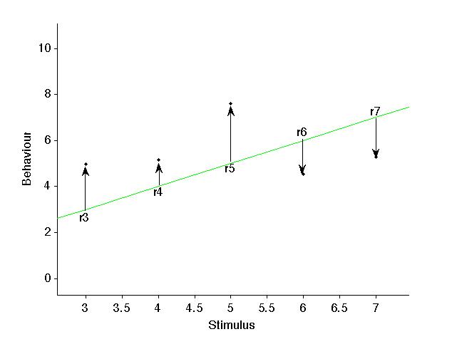
But why are some lines better than others? Because they 'go through the data better' - in other words they minimise the overall distance between the line and the data points. This can be measured by taking the sum of square errors (SSE) - a fancy way of saying 'measure the distance from the line to each data point, square each distance and add them all together'

SSE = r1² + r2² + r3² + r4² ... + r10²

Measuring the errors

The important thing to realise is that the SSE quantifies how good the fit is, and that there is a value of SSE for every possible slope. The task of least-squares regression is to find the slope that minimises the SSE. But note that there is no slope that is "right" - we're just trying to find the one that is least wrong.

Every slope has its own quality of fit

Here the best fit line is found to have a slope of about 1.1, which is close the the slope of 1 that I used to make the data. Notice how the SSE (the total error) gets bigger as we move away from the best fit - making the line either steeper or shallower increases the error, which means that the fit is worse.

By seeing how quickly the fit gets worse when we change the slope we can estimate how certain we are about the best fit - if there is a wide area where the SSE is almost the same at the bottom then there are lots of slopes that are almost-as-good as the best line, which tells us that the data isn't enough to estimate the function well.

It is important to see that we could find the best slope without using a special formula. We could simply use trial and error, calculating the SSE for one slope, then another, moving in the same direction if the SSE improves and going back if it gets worse. Or we could do what I did to plot that figure and simply try lots of possible values of the slope and find the SSE for each one. When we start fitting more complicated functions we won't always have a nice neat formula that tells us what the best fit will be.

In the next post we'll look at how linear regression can be used for more than one stimulus and how we can fit non-linear functions.

How Fish Shoal (1): Understanding Regression

In late 2011 our research group at Uppsala University and our colleagues at the University of Sydney, published a study that aimed to show how fish in shoals change their speed and direction of movement in response to the other fish. We had placed groups of fish together in a tank and tracked their movements (see video below). How do we get from that to understanding how they respond to each other?



Let us begin by asking what we mean by saying 'we understand' why a fish changes its motion. My definition is that I understand why a fish does this if I can predict it. That is, I can say what a fish will do next if I know what its environment is like (I'm leaving the exact definition of 'the environment' intentionally vague at this point).

Environment → Next Behaviour

Mathematically we call this finding a mapping between the things on the left and the things on the right. We often write a mapping as a function, f.


Next Behaviour = f(Environment)

Understanding requires us to find how the environment influences behaviour. That is, we must find out what the function, f, is.

Having defined our goal, our next task is to make things a little more concrete. What behaviours are we interested in predicting? Which aspects of the environment do we think could be important? We chose to try to predict how a fish will change its speed and direction, using the positions and directions of the other fish around it. Let us consider only the change of speed, we now want to find a function such that:

speed change = f(positions of other fish, directions of other fish)

Now these are things we can actually measure from the recorded tracks (see figure below). So we can say where, for example, the nearest fish to our focal fish was at each moment, and correspondingly how much the focal fish accelerated or decelerated at that moment.

Measuring the position of the nearest fish

So have data giving both the inputs to the function (the positions/directions of the other fish), and the output (the acceleration of the focal fish). How do we learn what the function is. This task is generally known as regression. You will almost certainly have come across linear regression at school, which is a special case of this method, but generally regression simply means learning how one variable predicts another. Specifically we use the term 'regression' in contrast to 'classification': regression is used when we are dealing with a output (such as the acceleration) that can take many values. Classification is used for either/or type outputs, such a whether someone recovers from a disease.

In the next post we'll see how we can use our data to learn what the function mapping the environment to behaviour looks like, starting by recapping on the principles of linear regression...